Market simulation

The purpose of this tutorial is to show a more in-depth guide on how to simulate a market using Garpar, along with all the available tweaks for the process.

Currently, the system supports market simulation using one of the following distributions: normal, uniform, or Lévy stable. We will use the normal distribution for this tutorial.

We can run our first simulation by doing the following:

from garpar.datasets.risso import make_risso_normal

make_risso_normal()

Stocks	S0[W 1.0, H 0.5]	S1[W 1.0, H 0.5]	S2[W 1.0, H 0.5]	S3[W 1.0, H 0.5]	S4[W 1.0, H 0.5]	S5[W 1.0, H 0.5]	S6[W 1.0, H 0.5]	S7[W 1.0, H 0.5]	S8[W 1.0, H 0.5]	S9[W 1.0, H 0.5]
Days
0	100.000000	100.000000	100.000000	100.000000	100.000000	100.000000	100.000000	100.000000	100.000000	100.000000
1	99.130675	98.938457	100.957522	101.055805	100.833733	98.988901	100.918242	100.998449	101.201640	99.138093
2	98.178339	97.784901	102.287085	101.949808	101.958618	98.044692	99.715934	102.213639	102.437984	100.151271
3	97.095716	96.951917	101.162984	102.838534	103.188705	97.222261	100.978839	101.515875	103.425717	101.162765
4	95.998882	95.960271	100.397372	104.138974	104.270481	95.876879	101.791423	100.261614	102.747004	102.203154
...	...	...	...	...	...	...	...	...	...	...
361	103.020396	119.635710	137.069866	105.605818	97.820445	96.309881	108.971972	109.696736	130.341584	114.169307
362	103.721805	118.662972	138.319683	107.053940	98.937359	95.098037	107.680058	108.283752	129.077786	115.315552
363	104.802485	119.592428	136.678404	106.061436	99.632836	95.401246	106.875893	107.661266	128.131457	116.618105
364	106.149640	118.655703	138.284264	107.406245	101.020342	96.480746	107.960867	108.712707	129.569422	115.835380
365	105.013537	120.034767	136.894239	106.466550	99.769447	97.429199	109.256713	107.328981	128.137076	114.517254

366 days x 10 stocks - W.Size 5

By default, the simulation generates 10 stocks with 365 days of prices for each one. These prices follow the same distribution.

For this tutorial, we will focus on three sections of the StocksSet:

1. Entropy (H): Located in the top section, representing the entropy of the prices of each stock. By default, this value is 0.5.

2. Stock Prices: The section that displays the value of each stock for each day.

3. Market Data: Found at the bottom, this section includes:

   • Total days

   • Number of stocks

   • Window size (we will explain its significance as we progress).

Parameters of a Simulation

There are several parameters that influence a simulation. This section will demonstrate how each parameter affects the results.

Let’s start with a simple example. Suppose we want to simulate 5 stocks over 10 days, each starting at a price of 110. This can be achieved with the following function call:

make_risso_normal(days=10, stocks=5, price=110)

Stocks	S0[W 1.0, H 0.5]	S1[W 1.0, H 0.5]	S2[W 1.0, H 0.5]	S3[W 1.0, H 0.5]	S4[W 1.0, H 0.5]
Days
0	110.000000	110.000000	110.000000	110.000000	110.000000
1	109.117728	111.142480	109.005964	111.225238	108.933941
2	108.148428	109.991785	108.061761	110.292676	107.964431
3	106.781601	109.049845	106.585629	109.216555	108.731131
4	108.099429	110.075661	107.907369	108.120015	109.657296
5	107.252916	110.952404	108.953459	107.277810	108.505686
6	106.360039	109.793367	107.872222	105.925655	107.491105
7	105.230028	110.939719	106.961106	106.767284	106.719316
8	106.280762	109.639860	108.318413	105.770203	107.565712
9	105.290723	111.191792	107.490741	106.812023	106.613072
10	106.481003	112.601400	108.828019	107.681678	105.136796

11 days x 5 stocks - W.Size 5

Sometimes, we might want a more ‘controlled’ or even deterministic environment. We can achieve this by using a seed. The random_state parameter represents this seed, as shown in the following example:

make_risso_normal(days=10, stocks=5, random_state=42)

Stocks	S0[W 1.0, H 0.5]	S1[W 1.0, H 0.5]	S2[W 1.0, H 0.5]	S3[W 1.0, H 0.5]	S4[W 1.0, H 0.5]
Days
0	100.000000	100.000000	100.000000	100.000000	100.000000
1	98.805864	100.935769	99.326480	100.900464	100.649803
2	99.723073	99.709073	98.300671	99.884634	101.809271
3	100.481068	98.845525	99.570943	98.878556	100.721910
4	99.870674	97.846148	100.461281	99.783308	99.528206
5	101.124337	96.897283	101.310699	98.637364	100.581171
6	102.006936	95.770467	100.074504	99.746865	101.208367
7	103.332098	94.844957	101.280570	100.450735	100.356336
8	104.518001	94.306958	102.217987	99.473017	101.303750
9	105.458859	93.176509	100.824345	100.715559	100.136298
10	106.641517	92.403867	101.862962	99.497536	99.235579

11 days x 5 stocks - W.Size 5

Feel free to try this with different values of random_state.

Now, let’s talk about the H value. This represents the entropy of a given stock, which can be thought of as the informational efficiency of the market. In simple terms, it describes how quickly information spreads throughout the market. Entropy is essentially a measure of unpredictability. When the entropy value is closer to 1.0, it means that the chances of winning or losing on any given day are nearly equal—making the stock’s movements highly unpredictable. On the other hand, when entropy is closer to 0.0, it suggests that the chances of winning or losing are imbalanced, meaning the stock’s behavior is more predictable or skewed in one direction.

To test this, lets try using a high entropy value and a low entropy value. This will show how this concept is visualized:

make_risso_normal(stocks=1, entropy=1.0, random_state=702).plot.line(
    palette="flare"
)
make_risso_normal(stocks=1, entropy=0.0, random_state=702).plot.line(
    palette="viridis"
)

<Axes: title={'center': 'Price'}, xlabel='Days'>

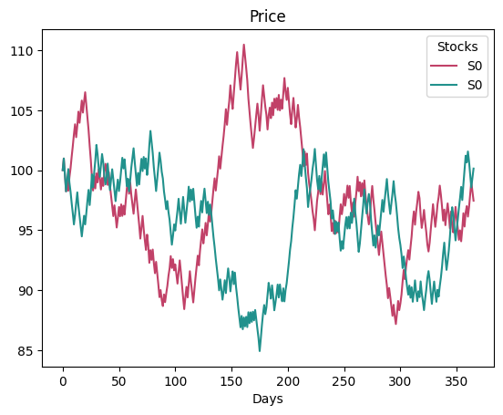
We can see that the stock following the red line doesn’t show a clear, sustained trend of either dropping or rising, while the one with the teal color tends to drop over time.

Note that we used a method line to create the graph, the attribute plot is known as an accessor and we will explain them in one of the lasts sections of this tutorial.

Another important parameter is the window_size, which represents how long an investor will hold a stock. By default, we’ve set it to 5 days. This value is combined with the entropy to determine the loss probability each day. So for example, lets assume the same entropy value and see how the stocks values diverge:

make_risso_normal(
    stocks=1, entropy=0.5, window_size=5, random_state=702
).plot.line(palette="flare")
make_risso_normal(
    stocks=1, entropy=0.5, window_size=7, random_state=702
).plot.line(palette="viridis")

<Axes: title={'center': 'Price'}, xlabel='Days'>

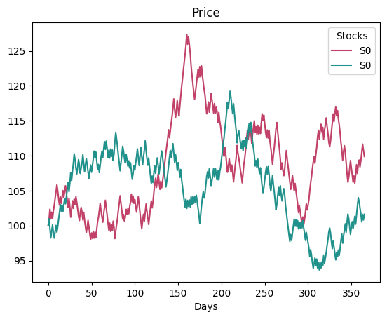
As we can see, the simulation produces different results based on the window_size.

We’ve also included some validations. For example, if we try to simulate a market with fewer days than the window_size, the simulation will fail. In such cases, we issue a warning to inform the user about what’s happening:

make_risso_normal(days=10, stocks=4, random_state=42, window_size=20)

---------------------------------------------------------------------------
ValueError                                Traceback (most recent call last)
Cell In[6], line 1
----> 1 make_risso_normal(days=10, stocks=4, random_state=42, window_size=20)

File ~/checkouts/readthedocs.org/user_builds/garpar/envs/stable/lib/python3.12/site-packages/garpar/datasets/risso.py:384, in make_risso_normal(mu, sigma, entropy, random_state, n_jobs, verbose, **kwargs)
    344 """Create a StocksSet instance using RissoNormal maker.
    345
    346 This function is intended to create a StocksSet instance using the
   (...)    373     Generated stocks set instance.
    374 """
    375 maker = RissoNormal(
    376     mu=mu,
    377     sigma=sigma,
   (...)    381     verbose=verbose,
    382 )
--> 384 return maker.make_stocks_set(**kwargs)

File ~/checkouts/readthedocs.org/user_builds/garpar/envs/stable/lib/python3.12/site-packages/garpar/datasets/ds_base.py:349, in RandomEntropyStocksSetMakerABC.make_stocks_set(self, window_size, days, stocks, price, weights)
    326 """Create a StocksSet instance with random prices.
    327
    328 Parameters
   (...)    346
    347 """
    348 if window_size <= 0 or window_size > days:
--> 349     raise ValueError("'window_size' must be in the interval (0, days]")
    351 initial_prices = self._coerce_price(stocks, price)
    353 loss_probability = self.get_window_loss_probability(
    354     window_size, self.entropy
    355 )

ValueError: 'window_size' must be in the interval (0, days]

As we mentioned, there are other distributions that a market prices follow. Feel free to test them. In the current version we have the functions make_risso_unifom and make_risso_levy_stable appart from the make_risso_normal shown in the previous steps.

There are other parameters that can be used in a simulation, such as n_jobs, which represents the number of concurrent ‘workers’ used for the simulation, or the verbose parameter, which, when set to 1, shows details of such ‘workers’.

Combining simulations

We can use the make_multisector function to run the simulation with different distribution or simulation values at the same time. For example, if we want to see how the prices change with a particular seed and the three distributions, we can do something like the following:

from garpar.datasets import (
    RissoUniform,
    RissoNormal,
    RissoLevyStable,
    make_multisector,
)

make_multisector(
    RissoNormal(random_state=42),
    RissoUniform(random_state=42),
    RissoLevyStable(random_state=42),
    days=10,
    stocks=3,
)

Stocks	rissonormal_S0[W 1.0, H 0.5]	rissouniform_S0[W 1.0, H 0.5]	rissolevystable_S0[W 1.0, H 0.5]
Days
0	100.000000	100.000000	100.000000
1	98.805864	97.632493	99.783564
2	99.723073	101.690331	100.449422
3	100.481068	105.711307	101.042132
4	99.870674	100.473104	100.711882
5	101.124337	104.818773	102.554182
6	102.006936	108.857429	103.839387
7	103.332098	114.204546	104.271329
8	104.518001	118.185062	106.170553
9	105.458859	120.886469	106.377469
10	106.641517	122.287369	106.493258

11 days x 3 stocks - W.Size 5

The classes RissoUniform, RissoNormal and RissoLevyStable are known as makers in our system. Objects of these classes are in charge of creating StocksSet, the difference between each one is the distribution a generated StocksSet prices follow.

The accessors

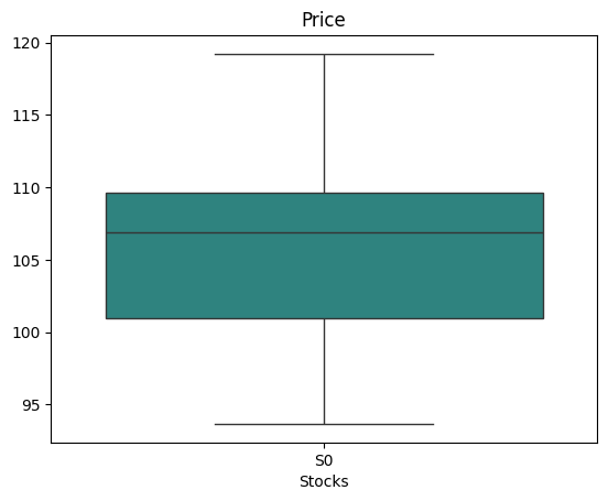
The accessors are properties that allow an object to be treated as a particular tipe. When we introduce the entropy value, we utilized the property plot, this property had an interface inside to make different plots of the StocksSet. We used only the line plot, but if we want to make a boxplot; we will simply make something like this:

make_risso_normal(
    stocks=1, entropy=0.5, window_size=7, random_state=702
).plot.box(palette="viridis")

<Axes: title={'center': 'Price'}, xlabel='Stocks'>

There are many other accessors. Feel free to look for the Core subpackage in the API section, where we published every function prototype alongside its documentation!

Now that you know how the simulation works, we recommend you to follow this tutorial.